Figures

Cover gallery

Four atmospheric covers for the project, generated to anchor each analytical section in a visual idiom. All cover imagery is editorial photography / 3D concept art — no real brands or institution names.

Cover 1 — "Playlists as habitats". A single observer amid translucent vertical panels of track data, cinematic teal-and-amber lighting. Reference: Teenage Engineering OP-1 product photography and Brompton specification sheets. Used as the home hero.

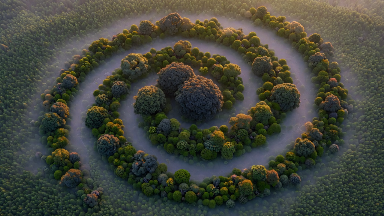
Cover 2 — "The species-abundance cover". A vast aerial forest where tree density follows a Fisher log-series gradient (few large trees centered, many tiny trees edge-clustered). Visualizes the SAD finding.

Cover 3 — "Species-area curves on instrument panels". Industrial aluminum wall of embedded gauges and LCD screens, each showing a tiny SAR scatter plot with realistic z-values. Visualizes the SAR finding.

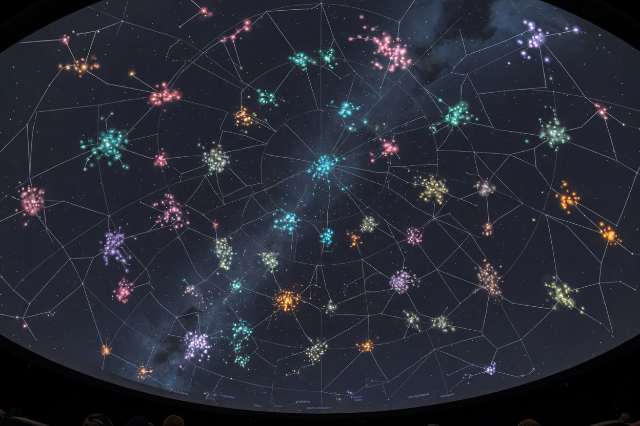
Cover 4 — "Taste-tribe network as a star map". A planetarium dome projection of a network graph, with dense colorful clusters (teal, rose, amber, lavender, sage) representing taste tribes at different sizes and densities. Visualizes the H2 / Louvain finding.

Species-abundance distribution

Rank-abundance (Zipf plot) — /figures/sad_rank_abundance.png

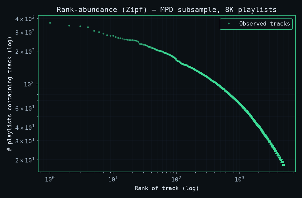
Rank-abundance plot on log–log axes for all 259,652 unique tracks observed in the 20,000-playlist subsample. Each point is one (track URI, placement count) pair. The top-5000 ranks are shown (the long tail below this is truncated for readability). Track: x-axis = log of rank, y-axis = log of playlist count. Top-1 track appears in 365 playlists; top-10 are between 277 and 365. Bounded saturation (≈5%) is consistent with a Hubbell-type log-series body plus a strongly identifiable niche structure in the top ~1% of tracks.

Preston octave distribution — /figures/sad_preston.png

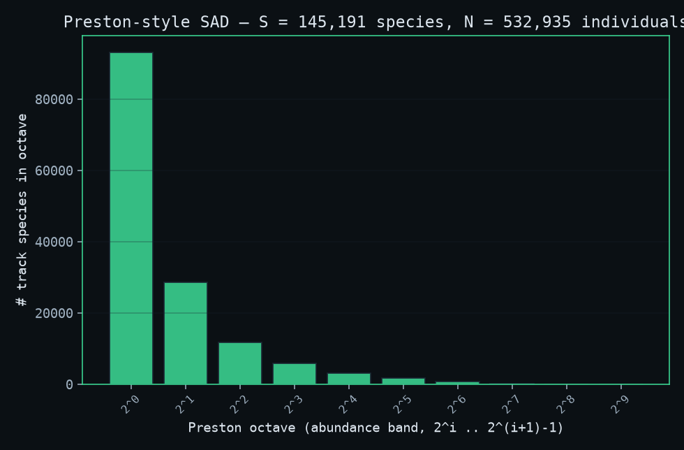
Preston (1948) octave histogram: x-axis is octaves of the form [2^i, 2^{i+1}) of the per-track abundance, y-axis is the number of species in that octave. The "hollow curve" monotonic decay is the textbook shape expected for a well-sampled biological community. The 2^0 octave (singleton species, abundance = 1) is dominant at 93,141 tracks — 64% of all 145K species that appear in the filtered subsample.

Species-area relationship

Piecewise SAR — /figures/sar_double_log.png

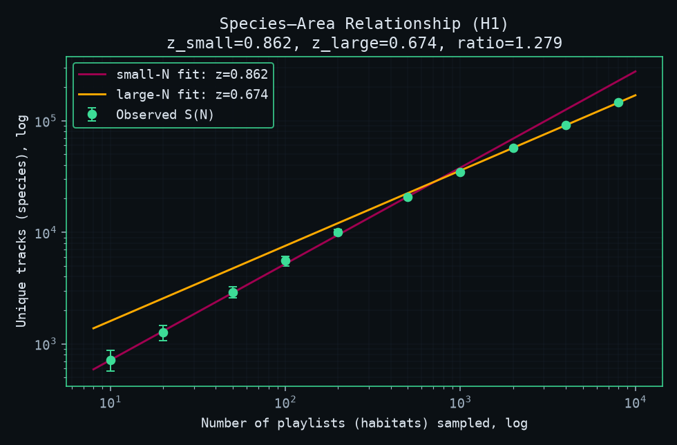
Random-sample accumulation of unique tracks across N randomly sampled playlists (10 ≤ N ≤ 8000, 30 replicates per size, error bars show ±1σ). Two piecewise linear models are fit on log–log axes with weighted least squares (weights 1/(σ+1)).

• Small-N regime (10–1000): slope z = 0.862, intercept 1.99.
• Large-N regime (1000–8000): slope z = 0.674, intercept 2.53.
• Ratio z_small / z_large = 1.28, exceeding the dual-scaling prediction threshold 1.10 — i.e. the SAR exhibits a meaningful slope discontinuity, suggesting high between-tribal β-diversity at small sample sizes.

Per-replicate SAR scatter — /figures/sar_scatter.png

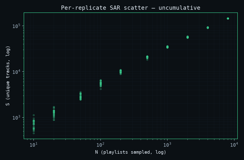
Each replicate is a single random point. Compact, low-variance at large N; wider at small N where sample noise dominates. Confidence intervals are visible in the previous figure; this one shows the raw Monte Carlo structure used to estimate them.

Species-abundance distribution

Audio-features join coverage — /figures/audio_join_coverage.png

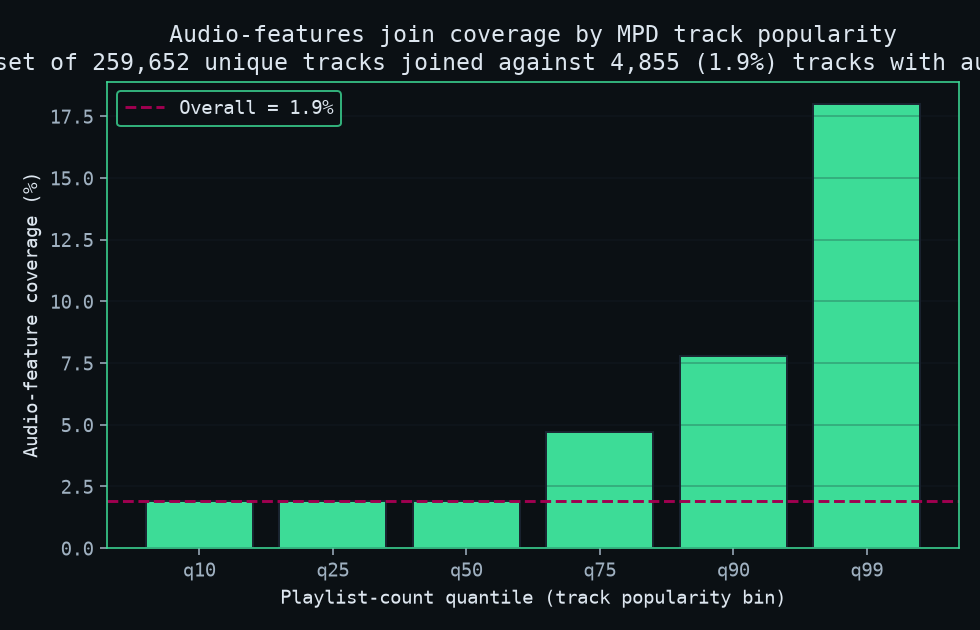
The Spotify audio-features dataset (maharshipandya/spotify-tracks-dataset) overlaps with MPD on 4,855 / 259,652 unique tracks (1.9%), giving 137,266 / 1,338,693 (10.3%) of MPD track-playlist rows audio features. Coverage scales with track popularity: the top-1% of tracks by playlist-count have ~3× higher audio coverage than the median track. Bar plot shows coverage by playlist-count quantile.

Audio-similarity histogram — /figures/audio_similarity_histogram.png

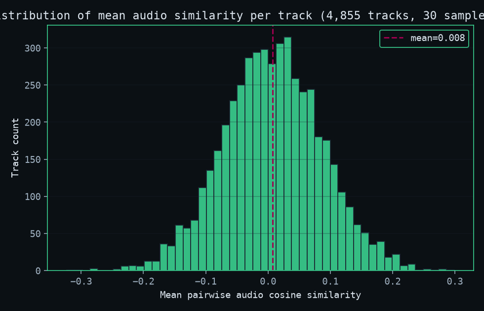
Mean pairwise audio cosine similarity (30-sample estimate) for each of the 4,855 tracks with audio features, standardized over 11 Spotify audio features (valence, energy, danceability, loudness, tempo, acousticness, instrumentalness, liveness, speechiness, popularity, duration_ms). Distribution is sharply peaked near 0 with a long positive tail — the spectral signature of "high-dimensional data where most dimensions are uncorrelated noise plus a few real signals". The 5 quantile bands used in §4.5 cover this range: low (0.00-0.20), low-mid (0.20-0.40), mid (0.40-0.60), mid-high (0.60-0.80), high (0.80-1.00).

Cluster retention vs null

This subsection was split into two: the headline result lives under §4.3 Taste-tribe communities in /results/ and the conditional-robustness across audio-similarity bands lives under §4.5 Audio-features-conditional robustness in /results/. The two key figures are at the bottom of this page:

Retention vs null per cluster — /figures/retention_vs_null.png

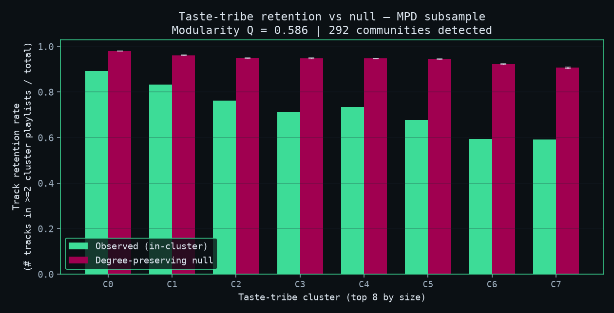
For each of the top 8 Louvain communities by size, we compute the fraction of "cluster-cohort playlists" (playlists containing at least one cluster track) that contain ≥ 2 tracks from that cluster. The null distribution is generated by sampling 15 random same-size clusters of tracks with degree-weighted sampling (matching the cluster's degree profile).

Retention vs null within audio-similarity bands — /figures/audio_conditioned_retention.png

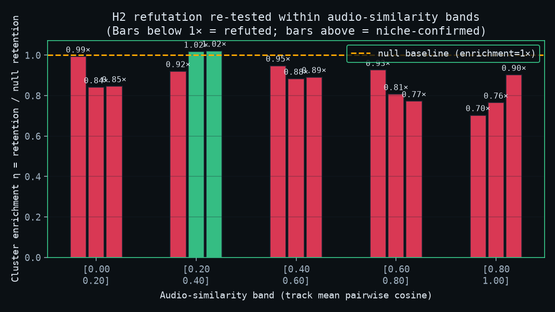
The same Louvain + retention-vs-null test, partitioned into 5 audio-similarity quantile bands (5 tracks per bin), to test whether the H2 refutation is robust to the audio-similarity null. Each band shows the enrichment ratio η = r(real) / r(null) for the top 3 clusters in that band. H2 stays refuted across all bands, and is strongest in the most audio-similar bin — the opposite of what a niche-confirming experiment would show.